|
FEBS ADVANCED COURSE: LIGAND BINDING, THEORY AND PRACTICE (Nove Hrady 3-10 July 2016) The scope of this practical exercise is to demonstrate how absorbance measurements can be used to determine equilibrium constants. This type of experiment has two requirements: (i) either the protein or the ligand needs to absorb UV or visible light. Given that UV/Vis photons have low energy, they are only able to promote electronic transition in the sample between relatively close energy levels. Typical UV/Vis chromophores have delocalized π orbitals and the light-excited quantum transitions are of the π --> π* type. Other types of quantum transitions (e.g. extraction of core electrons) require light of shorter wavelengths, down to the X rays. (ii) The chromophore must change its absorption properties (i.e. the energy leveles of its delocalized pi orbitals) upon ligation. Basic description of the method In UV/Vis absorption spectroscopy we measure the intensity of the light which is transmitted by the sample. We define: Transmittance: Ti = It,i/Iinc,i where It,i is the intensity of the light of wavelength i transmitted by the sample and Iinc,i that of the light incident on the sample (of the same wavelength). Obviously: 0 < T < 1. Absorbance: Ai = -log (Ti) Absorbance is directly correlated to the concentration of the absorbing chromophore by the law of Lambert and Beer: Ai = εi C L where εi is the extinction coefficient of the absorbing chromophore at wavelength i, C its concentration and L the length of the optical path (usually in cm). Typical extinction coefficients range between 0 and 150,000 M-1 cm-1. In practice we describe our reaction as P + X <==> PX, and summarize the requirements of our experiment as follows: (i) either the protein or the ligand must have ε > 0 (ii) the extinction coefficient of the chromophore should not be the same in the bound and free state, i.e. εP ≠ εPX or εX ≠ εPX It is advantageous if the following additional requirements are met: (iii) absorbance is due to the protein, not to the low molecular weight ligand, i.e. εP > 0, εX = 0 (iv) the ligand is perfectly soluble in the required concentration range. The experiment The binding of fluoride to met-myoglobin (ferric myoglobin) is accompanied by a large change in the extinction coefficient of the heme, which can be easily followed in the Soret band (450-390 nm). The reagents we prepared for this experiment are: buffer 0.1 M Tris/HCl pH=7.5 ferric horse myoglobin 60 uM in buffer sodium fluoride 0.5 M in buffer The expected Kd of fluoride is in the low mM range, and we want to explore a logarithmically spaced series of fluoride concentrations. Thus the following experimental design was implemented: 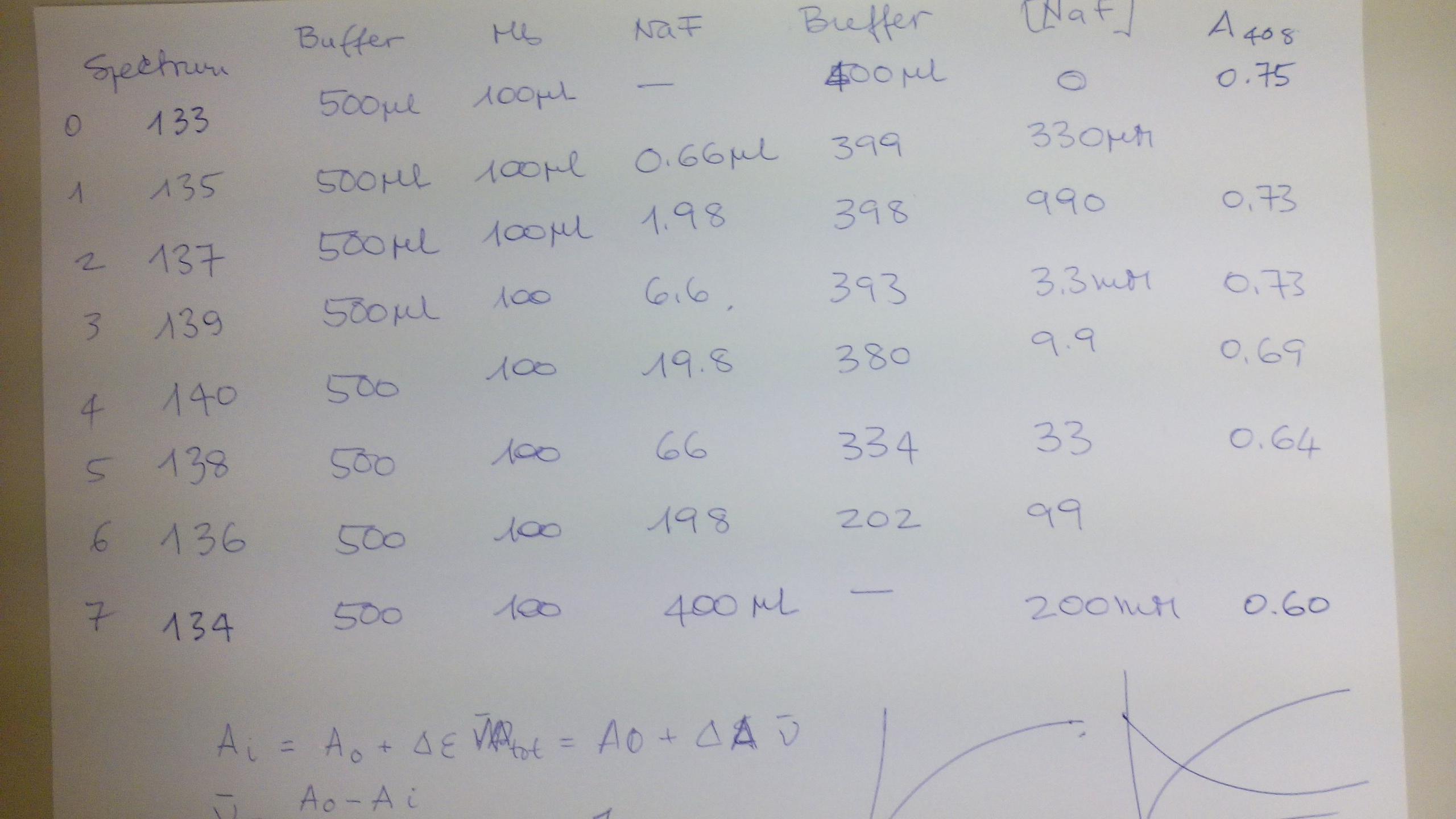
Samples were incubated 5 min. to allow the reaction to reach the equilibrium condition and the spectra were collecter in a Perkin Elmer Lambda 35 double beam spectrophotometer. This is how the samples look like: 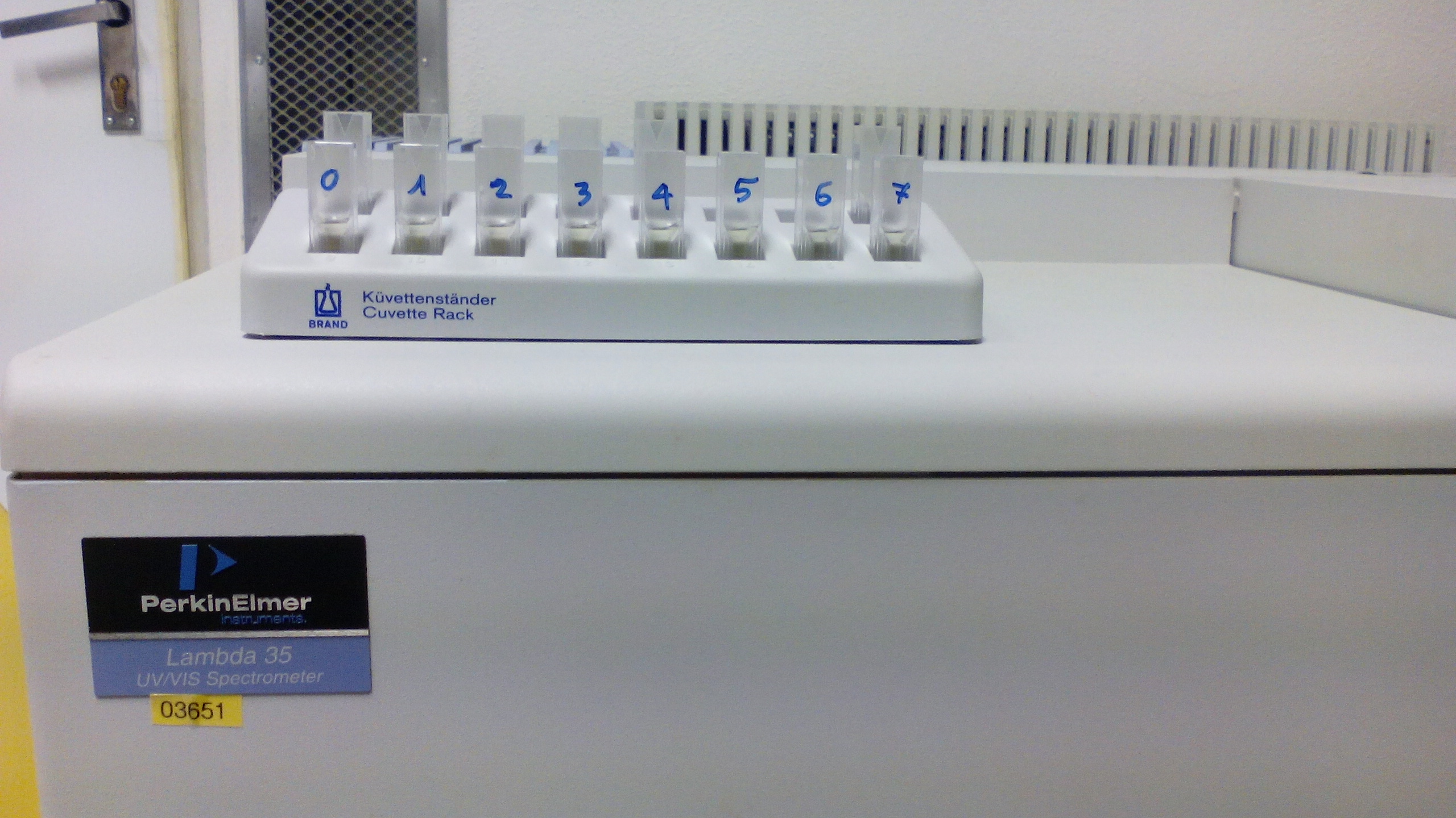
The spectra we collected were as follows: 
Analysis of the experimental data The analysis of the experimental data takes advantage of the additive property of Lambert and Beer's law. We can select the wavelenght at which the absorbance change is greatest (408 nm in our experiment) and write down the following equations: A = εP [P] L + εPX [PX] L Mass conservation dictates: [P]tot = [P] + [PX], thus we can substitute [P] with [P]tot - [PX], to obtain: A = εP [P]tot L + Δ εPX-P [PX] L and we recognize that: (i) εP [P]tot L represents the absorbance of the unliganded protein, before the addition of any ligand. We call this term A0. (ii) Δ εPX-P [PX] L may be rewritten as Δ εPX-P [P]tot ν L. Δ εPX-P [P]tot L equals the total absorbance difference we collected in our experiment; we call this term ΔA. Our equation rewrites as: A = A0 + ΔA [L]/([L]+Kd) We now have: a set of experimentally determined absorbances (at the wavelength we chosed as most suitable); and an equation that predicts the expected absorbance as a function of three parameters (A0, Δ A, and Kd) and one variable (the ligand's concentration). This allows us to plot the absorbance readings at 408 nm versus fluoride concentration and to compare them with the predicted absorbances, based on a single binding site equation: 
The data used to construct the above figure were as follows:
To improve our fitting of the equation to the experimental data (i.e. to find our best estimate of the model parameters), we need a computer program able to minimize the sum of the squared residuals: Σ (Aexp - Acalc)2 Limitations of the method To measure a Kd by means of Absorbance spectroscopy, we should be aware of the requirements and limitations of the method: (i) the free ligand concentration should be varied over a 4 log interval, centered on the Kd. The target, whose concentration is fixed, should be less concentrated than the ligand; this implis: [P]tot < Kd. (ii) However, the concentration of the chromophore (ideally the protein), is determined by its extinction coefficient since we want 0.1 < dA < 1 (approximately). This condition may not match with the above one: e.g. a weak chromophore may require concentrations higher than the Kd. (iii) Turbidity of the sample (e.g. because of protein precipitation) may cause baseline shifts. If small, these may be corrected by substituting single reading of absorbances with differences in the absorbance between two wavelengths of the each spectrum. Appendix: original absorbance readings (in case you want to analyze them)
|