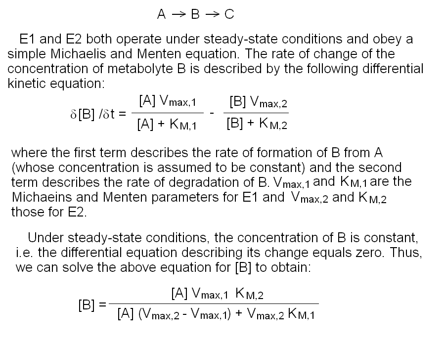
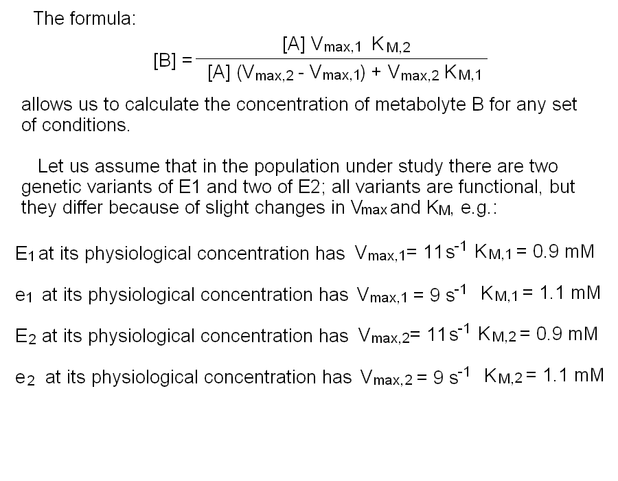
INTER-INDIVIDUAL VARIABILITY: AN EXERCISE
In this purely theoretical exercise, we shall investigate one among the possible causes of inter-individual variability.
Let us suppose that the terminal part of a metabolic pathway converts irreversibly metabolyte A into metabolyte B and then into terminal product C that is excreted. The reaction scheme is as follows: A --> B --> C
Reaction 1 irreversibly converts A to B and is catalyzed by enzyme E1; reaction irreversibly 2 converts B to C and is catalyzed by enzyme E2.
We further suppose that the concentration of metabolyte A is regulated by a negative feedback mechanism and is maintained constant. Moreover since product C is excreted and the reactions leading to its production are irreversible, we can neglect its concentration. We want to nvestigate the steady-state concentration of metabolyte B.
E1 and E2 both operate under steady-state conditions and obey a simple Michaelis and Menten equation. The rate of change of the concentration of metabolyte B is described by the following differential kinetic equation: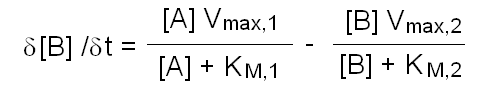

where the first term describes the rate of formation of B from A (whose concentration is assumed to be constant) and the second term describes the rate of degradation of B. V_max,1 and K_M,1 are the Michaelis and Menten parameters for E1 and V_max,2 and K_M,2 those for E2.

Under steady-state conditions, the concentration of B is constant, i.e. the differential equation describing its change equals zero. Thus, we can solve the above equation for [B] to obtain: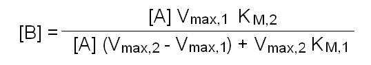

The above formula allows us to calculate the concentration of metabolyte B for any set of conditions.
Let us assume that in the population under study there are two genetic variants of E1 and two of E2, that we call E1, e1, E2 and e2 respectively. All variants are functional, but they differ because of slight changes in V_max and K_M, e.g.:

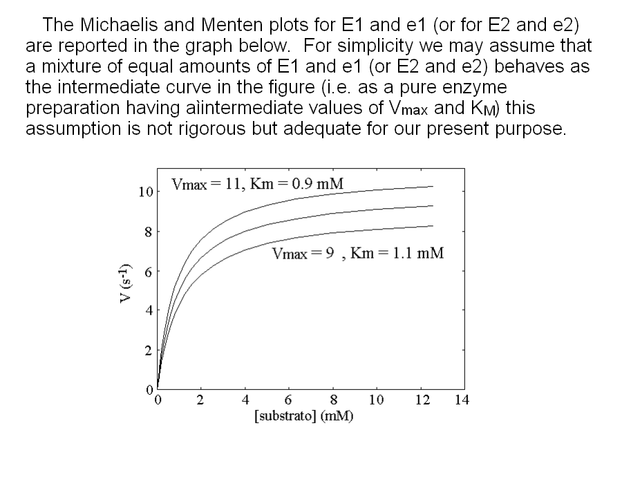
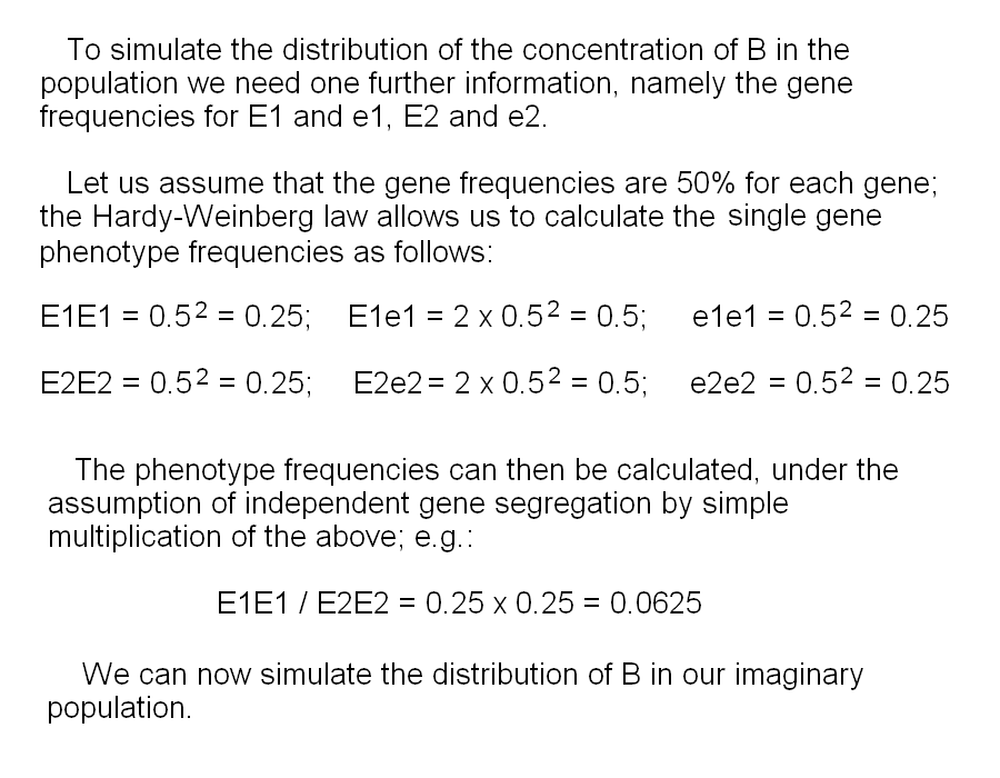
E1: V_max,1=11 s^-1; K_M,1=0.9 mM		e1: V_max,1=9 s^-1; K_M,1=1.1 mM
E2: V_max,2=11 s^-1; K_M,2=0.9 mM		e2: V_max,2=9 s^-1; K_M,2=1.1 mM

Let us further assume that the concentration of each enzyme is constant and that function of enzyme 1 in the heterozygous individual having an equimolar mixture of E1 and e1 can be approximated by a Michaelis and Menten equation with averaged parameters (i.e. V_max,1=10 s^-1; K_M,1=1 mM). The same applies to the function of enzyme 2. These approximations are very rough, but sufficient for our present purpose: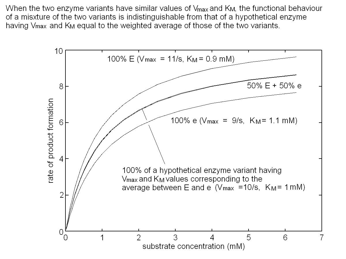

To simulate the distribution of the concentration of B in the population we need one further information, namely the gene frequencies for E1 and e1, E2 and e2. Let us assume that the gene frequencies are 50% for each gene; the Hardy-Weinberg law allows us to calculate the phenotype frequencies as follows:

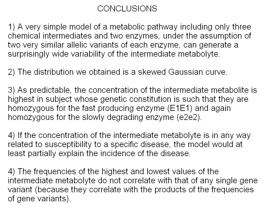
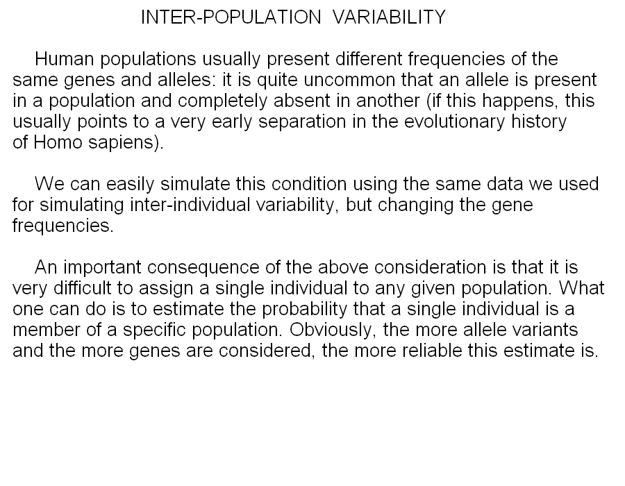
E1E1: 0.5²=0.25	E1e1: 0.5 x 0.5 x 2 = 0.5	e1e1: 0.5²=0.25
E2E2: 0.5²=0.25	E2e2: 0.5 x 0.5 x 2 = 0.5	e2e2: 0.5²=0.25

The frequencies of the different two-gene phenotypes are then calculated by multiplying those of the pertinent single-gene phenotypes; e.g.:
E1e1 / E2e2 = 0.5 x 0.5 = 0.25
The distribution of metabolyte B concentration in the population can be calculated as follows: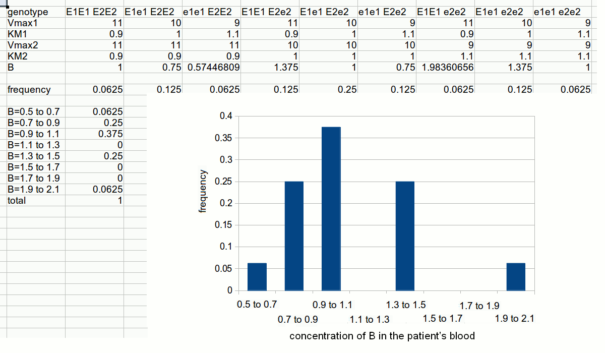

CONCLUSIONS 1) A very simple model of a metabolic pathway including only three chemical intermediates and two enzymes, under the assumption of two very similar allelic variants of each enzyme, can generate a surprisingly wide variability of the intermediate metabolyte.
2) The distribution of the intermediate metabolyte concentration is described by a skewed Gaussian curve.
3) As predictable, the concentration of the intermediate metabolyte is highest in subjects whose genetic constitution is such that they are homozygous for the more effective variant of the producing enzyme (E1E1), and again homozygous for the less effective variant of the degrading enzyme (e2e2).
4) If the concentration of the intermediate metabolyte is in any way related to susceptibility to a specific disease the model would partially explain the incidence of the disease.
5) The frequencies of the highest and lowest values of the intermediate metabolyte concentrations do not correlate with the frequency of any single gene variant (because they correlate with the products of the gene frequencies).

INTER-POPULATION VARIABILITY
Human populations usually present different frequencies of the same alleles of the same genes. It is quite uncommon that an allele is present in a population and completely absent in another (if this happens, this points to a very ancient separation in the evolutionary history of Homo sapiens).
We can easily simulate this condition using the same data we used for simulating inter-individual variability, but changing the gene frequencies. An important consequence of the above consideration is that it is very difficult to assign a single individual to any given population. What one can do is to estimate the probability that a single individual is a member of a given population. Obviously, the more allele variants and the more genes are considered, the more reliable this estimate is.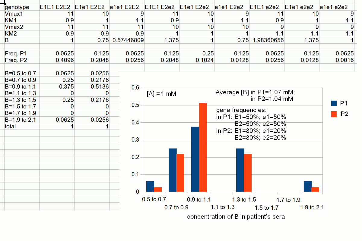

Slides of this lecture: