Course of LABORATORY MEDICINE
Statistical considerations
Diagnosis implies to assign a patient to a group, and requires a nosography, i.e. a coherent and comprehensive classification of diseases (e.g. the ICD). It will never be overemphasized that diagnosis is a complex process and that the recognition of the disease that affects the patient under study, and its correct classification, is only the first step. After this has been accomplished, the physician will ask why that specific patient succumbed to that disease, and which form that specific disease has taken in that patient: i.e. which specific and unique conditions are verified in each single case of disease. We may refer to these steps of the diagnostic procedure as the first (or general) and second (or individual) steps of diagnosis. From a historical point of view, the general perspective of diagnosis was initially suggested by Theophyle Laennec, strongly advocated by Robert Koch and finally formalized in modern terms by William Osler, the individual one by Archibald Garrod.
Because of interindividual variability (genetic, clinical, epidemiological) both steps of diagnosis are based on statistics: we infer something on a single patient because we can assign its case to a group and we know something on the group because of our previous experience. Thus not only the general diagnosis, but also the individual one is based on statistical reasoning. In what follows, we shall go through some basic concepts of statistics that have been largely dealt with in other courses.
HEALTH AND DISEASE
Diagnosing a disease in a patient implies that the physician has at least an intuitive concept of health and disease; unfortunately a precise definition of these terms is surprisingly difficult. I shall give here only some schematic considerations; the student may want to consult specialized treatises (e.g. E.A. Murphy, The Logic of Medicine or G. Canguilhem, Le Normal et le Pathologique).
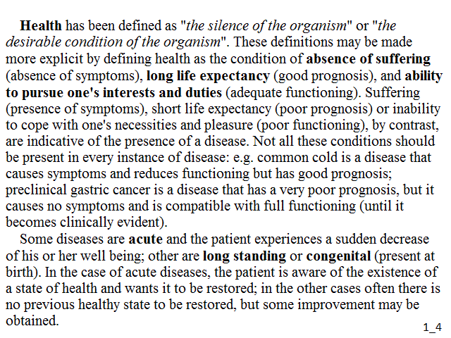
Health has been defined as "the silence of the organism" or "the desirable condition of the organism". These definitions may be made more explicit by defining health as the condition of absence of suffering (absence of symptoms), long life expectancy (good prognosis), and ability to pursue one's interests and duties (adequate functioning). Suffering (presence of symptoms), short life expectancy (poor prognosis) or inability to cope with one's necessities and pleasure (poor functioning), by contrast, are indicative of the presence of a disease. Not all these conditions should be present in every instance of disease: e.g. common cold is a disease that causes symptoms and reduces functioning but has good prognosis; preclinical gastric cancer is a disease that has a very poor prognosis, but it causes no symptoms and is compatible with full functioning (until it becomes clinically evident).
Some diseases are acute and the patient experiences a sudden decrease of his or her well being; other are long standing or congenital (present at birth). In the case of acute diseases, the patient is aware of the existence of a state of health and wants it to be restored; in the other cases often there is no previous healthy state to be restored, but some improvement may be obtained.
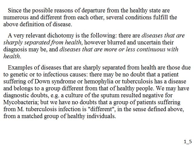
Since the possible reasons of departure from the healthy state are numerous and different from each other, several conditions fulfill the above definition of disease. A very relevant dichotomy is the following: there are diseases that are sharply separated from health, however blurred and uncertain their diagnosis may be, and diseases that are more or less continuous with health. Examples of diseases that are sharply separated from health are those due to genetic or to infectious causes: there may be no doubt that a patient suffering of Down syndrome or hemophylia or tuberculosis has a disease and belongs to a group different from that of healthy people. We may have diagnostic doubts, e.g. a culture of the sputum resulted negative for Mycobacteria; but we have no doubts that a group of patients suffering from M. tuberculosis infection is "different", in the sense defined above, from a matched group of healthy individuals.
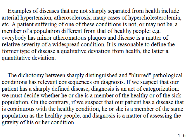
Examples of diseases that are not sharply separated from health include arterial hypertension, atherosclerosis, many cases of hypercholesterolemia, etc. A patient suffering of one of these conditions is not, or may not be, a member of a population different from that of healthy people: e.g. everybody has minor atheromatous plaques and disease is a matter of relative severity of a widespread condition. It is reasonable to define the former type of disease a qualitative deviation from health, the latter a quantitative deviation.
The above reasoning has relevant consequences on diagnosis. If we suspect that our patient has a sharply defined disease, diagnosis is an act of categorization: we must decide whether he or she is a member of the healthy or of the sick population. On the contrary, if we suspect that our patient has a disease that is continuous with the healthy condition, diagnosis is a matter of assessing the gravity of his or her condition.
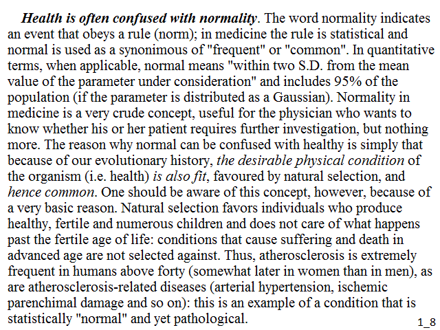
Health is often confused with normality. The word normality indicates an event that obeys a rule (norm); in medicine the rule is statistical and normal is used as a synonimous of "frequent" or "common". In quantitative terms, when applicable, normal means "within two S.D. from the mean value of the parameter under consideration" and includes 95% of the population (if the parameter is distributed as a Gaussian). Normality in medicine is a very crude concept, useful for the physician who wants to know whether his or her patient requires further investigation, but nothing more. The reason why normal can be confused with healthy is simply that because of our evolutionary history, the desirable physical condition of the organism (i.e. health) is also fit, favoured by natural selection, and hence common. One should be aware of this concept, however, because of a very basic reason. Natural selection favors individuals who produce healthy, fertile and numerous children and does not care of what happens past the fertile age of life: conditions that cause suffering and death in advanced ageare not selected against. Thus, atherosclerosis is extremely frequent in humans above forty (somewhat later in women than in men), as are atherosclerosis-related diseases (arterial hypertension, ischemic parenchimal damage and so on): this is an example of a condition that is statistically "normal" and yet pathological.
DISTRIBUTIONS: experimental error, homogeneous populations, heterogeneous populations
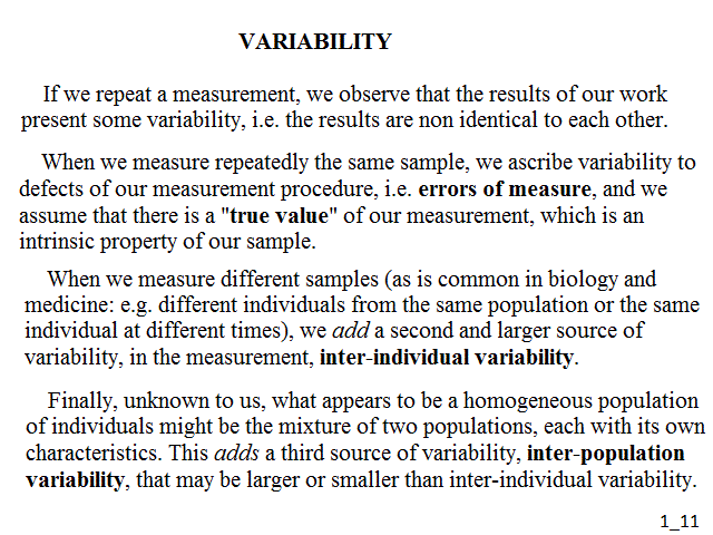
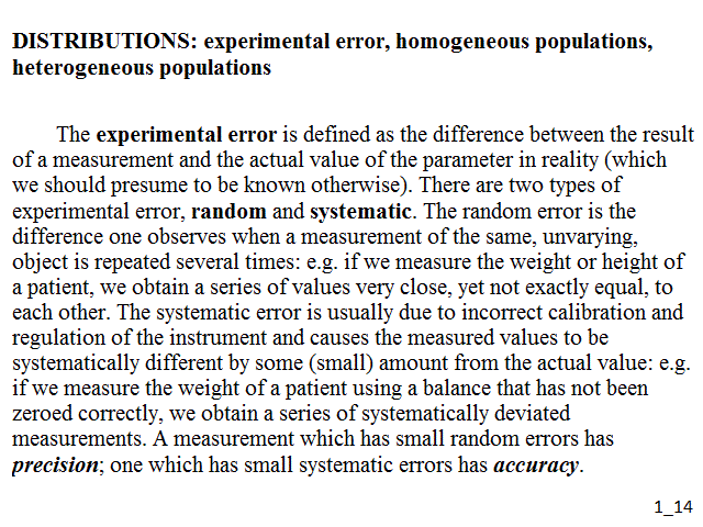
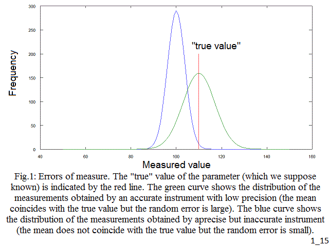
The experimental error is defined as the difference between the result of a measurement and the actual value of the parameter in reality (which we should presume to be known otherwise). There are two types of experimental error, random and systematic. The random error is the difference one observes when a measurement of the same, unvarying, object is repeated several times: e.g. if we measure the weight or height of a patient, we obtain a series of values very close, yet not exactly equal, to each other. The systematic error is usually due to incorrect calibration and regulation of the instrument and causes the measured values to be systematically different by some (small) amount from the actual value: e.g. if we measure the weight of a patient using a balance that has not been zeroed correctly, we obtain a series of systematically deviated measurements. A measurement which has small random errors has precision; one which has small systematic errors has accuracy.
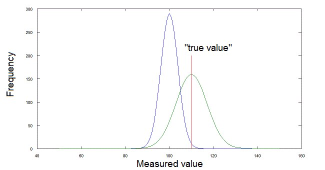
Fig.1: Errors of measure. The "true" value of the parameter (which we suppose known) is indicated by the red line. The green curve shows the distribution of the measurements obtained by an accurate instrument with low precision (the mean coincides with the true value but the random error is large). The blue curve shows the distribution of the measurements obtained by aprecise but inaccurate instrument (the mean does not coincide with the true value but the random error is small).
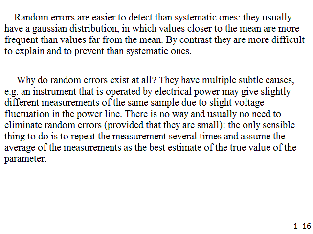
Random errors are easier to detect than systematic ones: they usually have a gaussian distribution, in which values closer to the mean are more frequent than values far from the mean. By contrast they are more difficult to explain and to prevent than systematic ones.
Why do random errors exist at all? They have multiple subtle causes, e.g. an instrument that is operated by electrical power may give slightly different measurements of the same sample due to slight voltage fluctuation in the power line. There is no way and usually no need to eliminate random errors (provided that they are small): the only sensible thing to do is to repeat the measurement several times and assume the average of the measurements as the best estimate of the true value of the parameter.
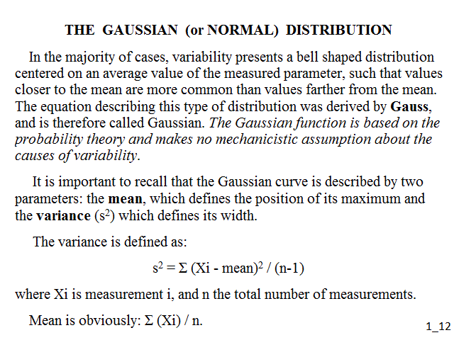
It is important to recall that the Gaussian (or bell-shaped) curve is described by two parameters: the mean, which defines the position of its maximum and the variance (s2) which defines its width. The variance is defined as:
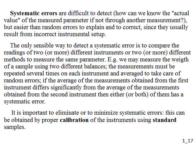
Systematic errors are difficult to detect (how can we know the "actual value" of the measured parameter if not through another measurement?), but easier than random errors to explain and to correct, since they usually result from incorrect instrumental setup. The only sensible way to detect a systematic error is to compare the readings of two (or more) different instruments or two (or more) different methods to measure the same parameter. E.g. we may measure the weigth of a sample using two different balances; the measurements must be repeated several times on each instrument and averaged to take care of random errors; if the average of the measurements obtained from the first instrument differs significantly from the average of the measurements obtained from the second instrument then either (or both) of them has a systematic error. It is important to eliminate or to minimize systematic errors: this can be obtained by proper calibration of the instruments using standard samples.
To estimate the systematic error of a clinical test is not an easy task. In some cases it can be done by preparing an artificial sample, using the most accurate and precise instruments in our laboratory and submitting it to the standard analysis. E.g. if we measure blood electrolytes using potentiometric methods, we can prepare a solution of the desired ion or salt at known concentration by weight (the balance is the most precise and reliable instrument in the lab), and submit it to the same potentiometric measure as our blood samples. We can also add the desired ion to the blood sample (by weighting appropriate amounts of a suitable salt) and measure its concentration (so called internal standard). Given the importance of this matter, all clinical instruments are frequently tested again known standards in order to check for random and systematic errors. An important point is the following: the relevance of systematic errors is minimized if the laboratory provides its own experimentally determined estimates of the "normal" range of the clinical parameters it measures (very few clinical laboratories do so). The reason is that the significance of clinical parameters is judged by comparison with their "normal" range and if both the parameter and its range are shifted in the same direction by a common systematic error, the significance of the measurement is not influenced by the error.
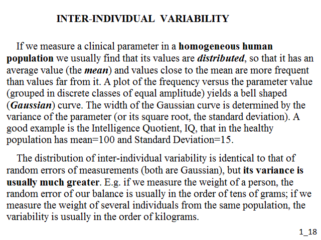
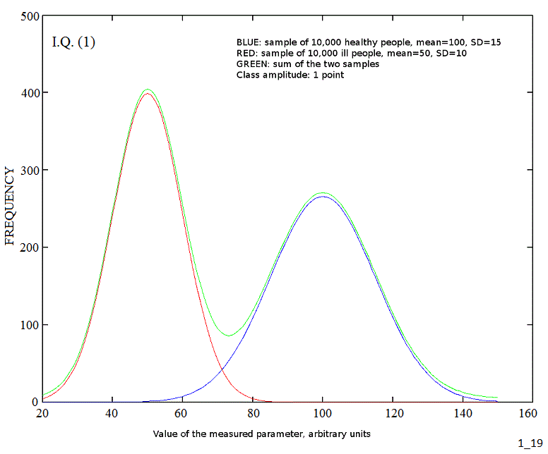
If we measure a clinical parameter in a homogeneous human population we usually find that its values are distributed, so that it has an average value (the mean) and values close to the mean are more frequent than values far from it. A plot of the frequency versus the parameter value (grouped in discrete classes of equal amplitude) yields a bell shaped (Gaussian) curve. The width of the Gaussian curve is determined by the variance of the parameter (or its square root, the standard deviation). A good example is the Intelligence Quotient, IQ, that in the healthy population has mean=100 and Standard Deviation=15 (see the blue curve in the figure below):
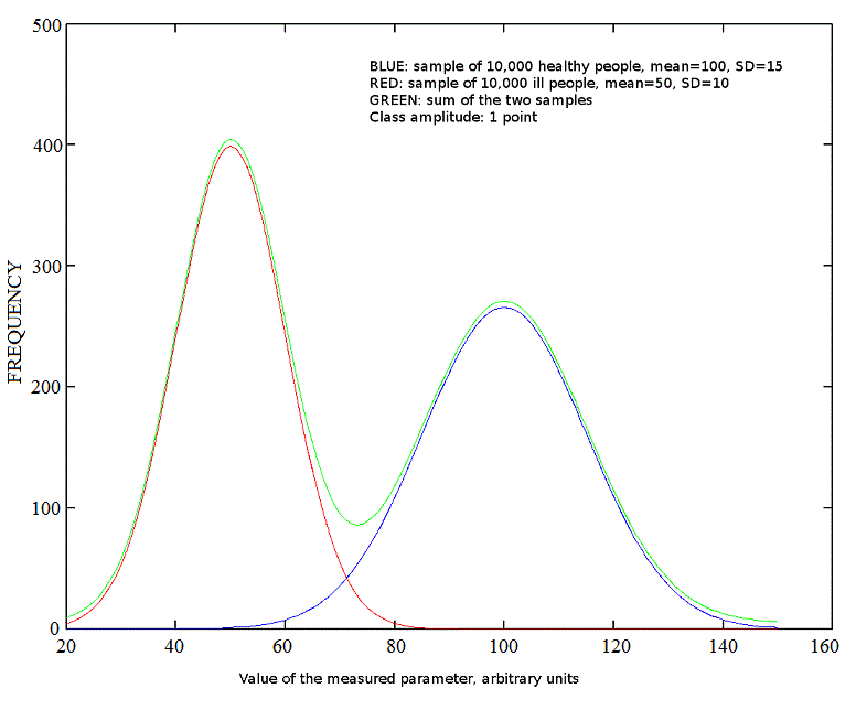
Fig.2: Gaussian distributions
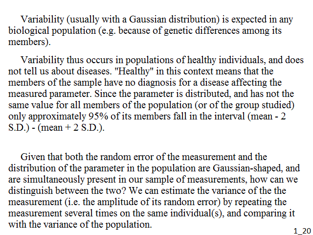
It is important to state that "healthy" in this context means that the members of the sample have no diagnosis for a disease affecting the measured parameter. Since the parameter is distributed, and has not the same value for all members of the population (or of the group studied) only approximately 95% of its members fall in the interval (mean - 2 S.D.) - (mean + 2 S.D.).
Given that both the random error of the measurement and the distribution of the parameter in the population are Gaussian-shaped, and are simultaneously present in our sample of measurements, how can we distinguish between the two? We can estimate the variance of the the measurement (i.e. the amplitude of its random error) by repeating the measurement several times on the same individual(s), and comparing it with the variance of the population. As a general rule, the variance of the measurement in the population is much greater than the that of the measurement on the same individual, and when dealing with the variance of the population, we can often neglect the random error of the measurement. The opposite case, i.e. that the variance of the population is as large as the variance of the measurement (it can never be smaller), is very uncommon and either indicates that the population is made up of identical members or that our instrument is too gross to detect the differences that are present.
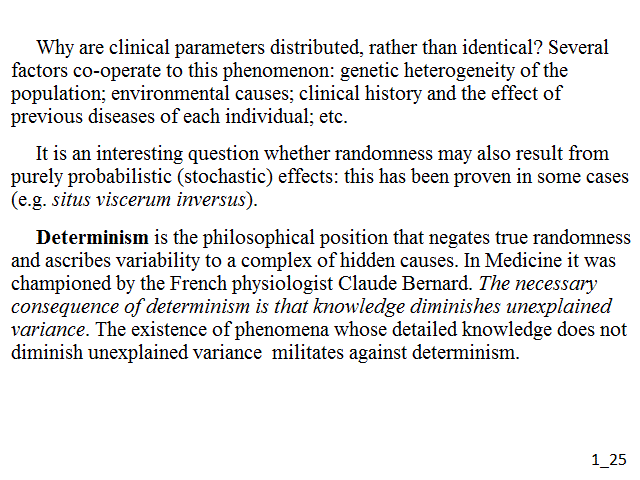
Why are clinical parameters distributed, rather than identical? Several factors co-operate to this phenomenon: genetic heterogeneity of the population; environmental causes; clinical history and the effect of previous diseases of each individual; etc. It is an interesting question whether randomness may also result from purely probabilistic (stochastic) effects: this has been proven in some cases (e.g. situs viscerum inversus).
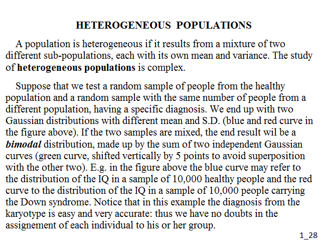
The case of heterogeneous populations is somewhat more complex. Suppose that we test a random sample of people from the healthy population and a random sample with the same number of people from a different population, having a specific diagnosis. We end up with two Gaussian distributions with different mean and S.D. (blue and red curve in the figure above). If the two samples are mixed, the end result wil be a bimodal distribution, made up by the sum of two independent Gaussian curves (green curve, shifted vertically by 5 points to avoid superposition with the other two). E.g. in the figure above the blue curve may refer to the distribution of the IQ in a sample of 10,000 healthy people and the red curve to the distribution of the IQ in a sample of 10,000 people carrying the Down syndrome. Notice that in this example the diagnosis from the karyotype is easy and very accurate: thus we have no doubts in the assignement of each individual to his or her group.
If we test a random sample from the human population, we shall include healthy and ill people according to the prevalence of each disease present in the population; and since ill people are usually much rarer than healthy, the distribution of the measured parameter will be again bimodal or multimodal, but the Gaussian curve corresponding to the healthy population will dominate the picture: e.g. the prevalence of all genetic defects leading to a mean IQ value of 50 or less is approximately 1% of the total population (see the red and blue curves in the picture below).
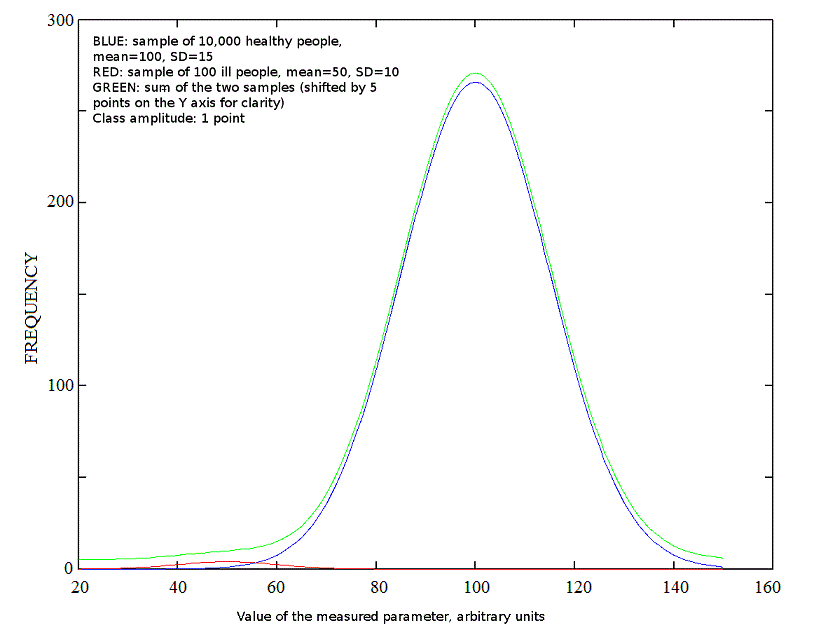
Fig.3: Gaussian distributions for populations of unequal amplitude
It will be noticed that in the above discussion of homogeneous aned heterogeneous populations, the problem of the experimental error in the measurements has been neglected: i.e. we have assumed that the random error is much smaller than the variance of the population and have taken the parameter values obtained from the clinical laboratory as precisely corresponding to the actual values in the patient. This assumption is usually safe: the experimental errors in the measurements are small with respect to the variability of the population. E.g. most measurements of concentration of blood solutes are accurate to within 2-3% of the actual value and when we say that the glycemia of a patient is 80 g/dL our confidence interval is in the order of 77-83 g/dL. However, not all clinical parameters have the same accuracy and we must be aware of possible errors in their measurement. Two conditions are special and require specific mention i.e.: (i) measurements that affect the value of the parameter of interest and (ii) the presence of confounding or interfering variables.
An example of a measurement that affects the parameter being measured is the recording of the blood pressure. In some individuals, the act of measuring the blood pressure causes psychological stress, and this in turn causes an autonomous response that increases the blood pressure (so called white coat hypertension). In this case we cannot resolve random and systematic errors of the measurement nor can we obtain a reliable estimate of the "normal" blood pressure of the patient. The best way to operate is to find a procedure that minimizes this effect (e.g. we can instruct the patient to measure his or her blood pressure by himself, using an automated recorder).
Confusing variables produce a signal indistinguishable from the variable of interest. E.g. the gravimetric measurement of oxalic acid in the urine is easily achieved by adding calcium chloride, allowing calcium oxalate to precipitate and weighting the dessiccated precipitate on a balance. This method is precise but if the urine contains any other anion whose calcium salt precipitates as well (e.g. phosphate) this will be confused with oxalate and will cause the amount of the latter to be overestimated. The presence of confusing variables should be carefully searched for, since they cause a systematic error difficult to detect; hopefully each test has a known and finite number of potential confusing variables (in some cases zero).
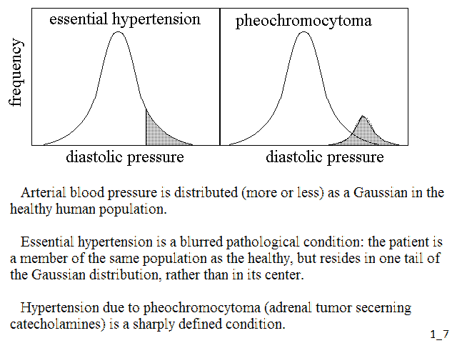
Some of the clinical parameters of a disease that is sharply distinguishable from the health condition will present a bimodal distribution in the general population: i.e. they will distribute in a (larger) Gaussian for the healthy group and a different (smaller) Gaussian for the sick group, even though some conditions (e.g. relative numerosities of the two groups) may mask the bimodality (Fig.3, above). In the case of diseases which are not sharply distinguished from the health condition, the distribution of the clinical parameters in the population is Gaussian and unimodal, and the disease group is identified as a "tail" of the distribution. An interesting example is that of arterial hypertension, that may be essential (i.e. idipathic, its cause being unknown), or may be due to some identified cause (e.g. pheochromocytoma). The corresponding distributions being as in Fig.4:
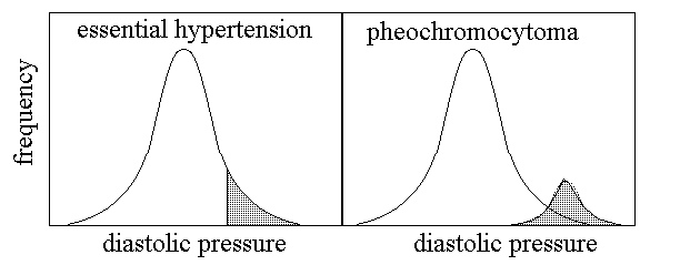
Fig.4: Distributions of diastolic pressure in the cases of essential hypertension and pheochromocytoma
How strong is the distinction between qualitative (i.e. sharply distinguished) and quantitative (i.e. continuous) deviations from the condition of health? Not very much. Indeed given that a quantitative deviation from health like essential hypertension has genetic and environmental factors, one may imagine that in the future we shall be able to identify precise causes and transform it into one or more sharply demarcated disease(s).
CERTAIN AND PROBABLE DIAGNOSES
Up to now we have considered the possible distributions of a measurable physiological parameter in the healthy, ill and mixed population, under the assumption that diagnosis could be made with certainty independently of our measurement. This is rarely the case: most often the parameter is a clue to the diagnosis, and we have to evaluate its clinical significance.
Before going further, let us distinguish diagnoses that are (almost) certain from diagnoses that are only probable. Some diseases are defined precisely enough to allow the physician to establish a diagnosis that is absolutely unequivocal. This is the case of most genetic diseases, e.g. the Down syndrome of the above example; of most infectious diseases, in which the presence of the causating agent can be demonstrated with certainty; of cancers, that can be ascertained bioptically; etc. In these cases the physiological parameters we measure give an indication for a definitive test, whose result confirms the diagnosis.
There are diseases in which an absolute diagnosis is impossible or at least not always possible. In general these diseases have no unequivocal histological or genetic marker (e.g. this is the case for most psychiatric diseases); moreover their cause is often unknown and several factors may cooperate; finally their gravity and prognosis may be highly variable (e.g. arterial hypertension). Even diseases which admit a certain and unequivocal diagnosis may under many instances be subject to uncertainty diagnosis: e.g. a cancer marker may be present in the blood of our patient but the tumour may be too small to be found and subjected to biopsy. In all these cases we formulate a probability diagnosis, i.e. we try to assess how likely it is that the patient is affected by a specific disease. Probability in this case estimates how confident we are in our diagnosis: the uncertainty lies in physician, not in the body of the patient; and we may increase our confidence by carrying out further tests.
MUPTIPLE DIAGNOSES
In some cases the patient suffers of more than a single disease and we must establish multiple diagnoses. Since the incidence of acute diseases is usually quite low and their duration is short, the coexistence in the same patient of two acute diseases independent of each other is an uncommon occurrence. By contrast the coexistance of two unrelated diseases one chronic, the other acute or both chronic is not infrequent, especially in the elder.
If we think that the patient suffers of two diseases at the same time, it is also important to establish whether or not they are correlated to each other: e.g. an acute episode of measles may cause the relapse of a previously silent tuberculosis. This is due to the temporary immunodeficiency due to measles that reduces the defences against the colonies of Mycobacterium tuberculosis already present in the lung or elsewhere in the body.
DISTRIBUTIONS IN RELATION TO DISEASES
As a general rule, when a disease admits an unequivocal diagnosis, its characteristic parameters exhibit a bimodal or multimodal distribution in the population, or, to be more rigorous, the human population is made up of a healthy and a hill subpopulation, each with its normal distribution of physiological parameters. The science philosopher Georges Canguilhem summarized this condition with the following definition: "there is a norm for health and one for (each) disease; and the two norms differ from each other". In these cases the physician uses the clinical parameters to assign his patient to its characteristic subpopulation. In the classical view of medicine, as championed by the great physicain William Osler, this assignement is the diagnosis. If and when a certainty diagnosis can be made, the two gaussians that represent the relevant diagnostic parameter in the healthy and ill groups are well separated from each other, with minimal or absent superposition: e.g. all patients suffering of Down syndrome have a trisomy of chromosome 21, at least a partial one; whereas all healthy people have no trisomy.
Diseases that only admit a probability diagnosis may take two very different forms:
(i) the relevant clinical parameter(s) have a bimodal distribution in the population, but the separation between the ill and healthy groups is incomplete (see the figures above); or
(ii) the relevant clinical parameter(s) have a monomodal, Gaussian distribution and the disease affects those individuals who present extreme values. An example of this condition is hypercholesterolemia.
The former condition is more frequent.
BAYESIAN STATISTICS
The most common condition faced by the clinician is the following: the patient presents some clinical parameters which are far from the mean value of the population, yet compatible with both illness and health (absence of a specific diagnosis). Is a diagnosis justified in his or her case? The answer to this question is a matter of probability and relies on the theory developed by the british mathematician Thomas Bayes (1702-1786).
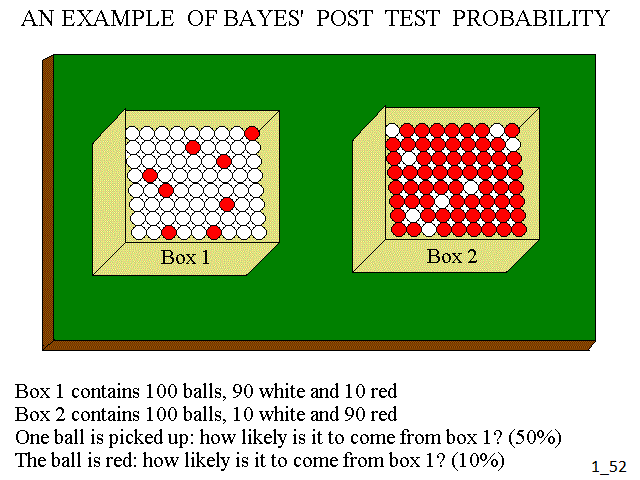
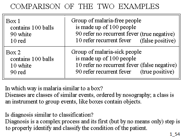
The textbook example of Bayes formula is the following: we have two boxes, each containing 100 balls. Box 1 contains 90 white and 10 red balls; box 2 contains 10 white and 90 red balls. One ball is picked up; how likely is it to come from box 1? This is the a priori probability and in the present case equals 50%, given that the two boxes contain the same number of balls and each has the same probability of being picked up. If we are told that the ball is red, can we refine our estimate? The answer is yes: since the ball is red, we ignore from our calculation all the white ones, and there are only 10% probability that the ball comes from box 1: this is because the system contains only 100 red balls, 10 in box 1 and 90 in box 2. Our new estimate is the ex post or post test probability. Often, we can add more tests and refine our estimate further.
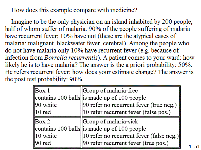
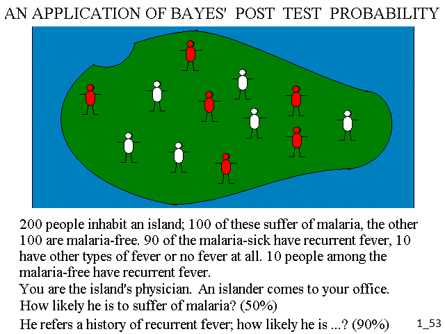
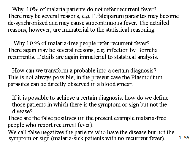
How does this example compare with medicine? Imagine to be the only physician on an island inhabited by 200 people, half of whom suffer of malaria. 90% of the people suffering of malaria have recurrent fever; 10% have not (these are the atypical cases of malaria: malignant, blackwater fever, cerebral). Among the people who do not have malaria only 10% have recurrent fever (e.g. because of infection from Borrelia recurrentis). A patient comes to your ward: how likely he is to have malaria? The answer is the a priori probability: 50%. He refers recurrent fever: how does your estimate change? The answer is the post test probability: 90%.
A comparison between the two examples is as follows:
| Box 1 contains 100 balls 90 white 10 red |
Group of malaria-free is made up of 100 people 90 refer no recurrent fever (true neg.) 10 refer recurrent fever (false pos.) |
| Box 2 contains 100 balls 10 white 90 red |
Group of malaria-sick is made up of 100 people 10 refer no recurrent fever (false neg.) 90 refer recurrent fever (true pos.) |
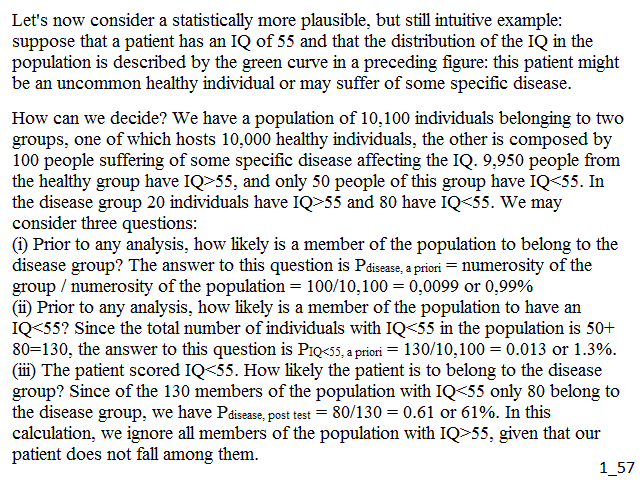
Let's now consider a statistically more plausible, but still intuitive example: suppose that a patient has an IQ of 55 and that the distribution of the IQ in the population is described by the green curve in Fig.2: this patient might be an uncommon healthy individual or may suffer of some specific disease. How can we decide? We have a population of 10,100 individuals belonging to two groups, one of which hosts 10,000 healthy individuals, the other is composed by 100 people suffering of some specific disease affecting the IQ. 9,950 people from the healthy group have IQ>55, and only 50 people of this group have IQ<55. In the disease group 20 individuals have IQ>55 and 80 have IQ<55. We may consider three questions:
(i) Prior to any analysis, how likely is a member of the population to belong to the disease group? The answer to this question is Pdisease, a priori = numerosity of the group / numerosity of the population = 100/10,100 = 0,0099 or 0,99%
(ii) Prior to any analysis, how likely is a member of the population to have an IQ<55? Since the total number of individuals with IQ<55 in the population is 50+80=130, the answer to this question is PIQ<55, a priori = 130/10,100 = 0.013 or 1.3%.
(iii) The patient scored IQ<55. How likely the patient is to belong to the disease group? Since of the 130 members of the population with IQ<55 only 80 belong to the disease group, we have Pdisease, post test = 80/130 = 0.61 or 61%. In this calculation, we ignore all members of the population with IQ>55, given that our patient does not fall among them.
The third question is our initial one: the likelyhood of a condition requiring diagnosis in the present case is 61%. The first and second questions have been considered to demonstrate the strength of our test, and because their answers will turn out useful in the following discussion.
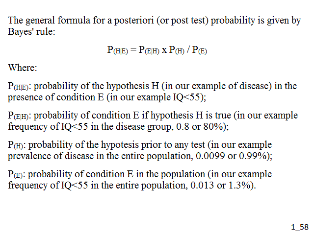
The general formula for a posteriori (or post test) probability is given by Bayes' rule:
P(H): probability of the hypotesis prior to any test (in our example prevalence of disease in the entire population, 0.0099 or 0.99%);
P(E|H): probability of condition E if hypothesis H is true (in our example frequency of IQ<55 in the disease group, 0.8 or 80%);
P(E): probability of condition E in the population (in our example frequency of IQ<55 in the entire population, 0.013 or 1.3%).
If we apply Bayes' formula to the data of our example we obtain:
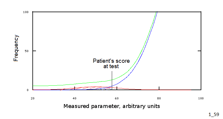
We may want to consider a graphical representation of our example: this is reported in figure 3 (which is an enlarged and modified portion of fig.2):
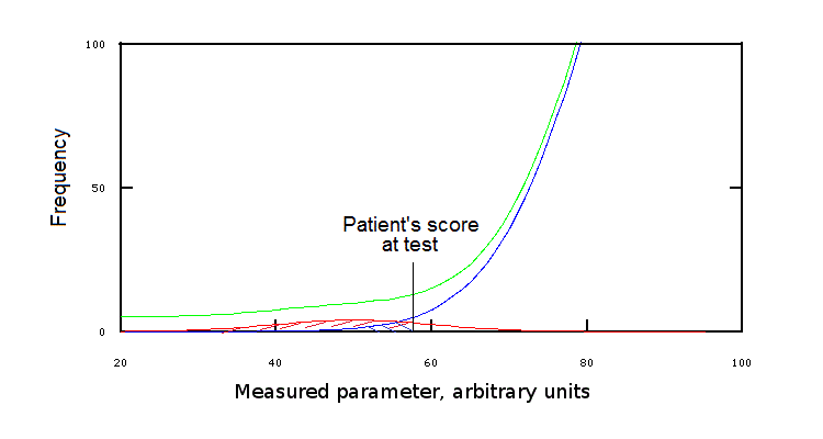
Fig.3: Position of the patient's score at test
Clearly, our example leaves something to be desired: indeed we arbitrarily divided our population and its groups according to the rule of thumb IQ<55, but we could greatly gain in precision setting a more precise condition, e.g. 50<IQ<60. However, Fig.3 makes it clear that, at least some values of the measured parameter, are compatible with both health and disease, even though with different probability.
Practical considerations on Bayes' formula
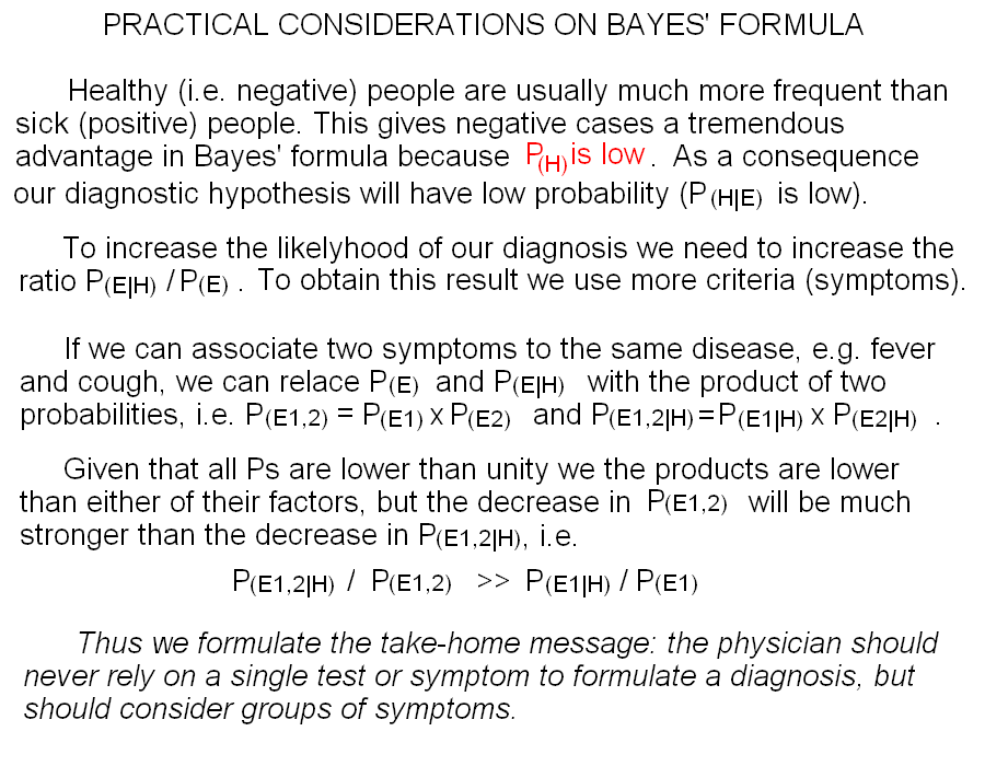
Healthy (i.e. negative) people are usually much more frequent than sick (positive) people. This gives negative cases a tremendous advantage in Bayes' formula because, no matter how strong the association between H (disease) and E (symptom)the absolute probability of H, P(H) is low. E.g. if the symptom is present in 99% of the cases of disease and in only 1% of the healthy population, but the frequency of disease is of 1 case in 10,000 population, Bayes' formula tells us that the probability of disease in a person presenting the symptom is Psub>(H/E) = 0.495. This follows from the fact that in a population of one million individuals there are 199 persons presenting the symptom, 99 affected by the disease and 100 healthy.
How can we increase the likelyhood of our diagnostic hypothesis? The answer is we need to increase the ratio P(E|H)/P(E). To obtain this result we use more criteria (symptoms). If we can associate two symptoms to the same disease, e.g. fever and cough, we can relace P(E) and P(E|H) with the product of two probabilities, i.e. P(E1,2)=P(E1)xP(E2) and P(E1,2|H)=P(E1|H)xP(E2|H). Given that all Ps are lower than unity we the products are lower than either of their factors, but the decrease in P(E1,2) will be much stronger than the decrease in P(E1,2|H), i.e. P(E1,2|H)/P(E1,2) >> P(E1|H)/P(E1).
Thus we formulate the take-home message: the physician should never rely on a single test or symptom to formulate a diagnosis, but should consider groups of symptoms.
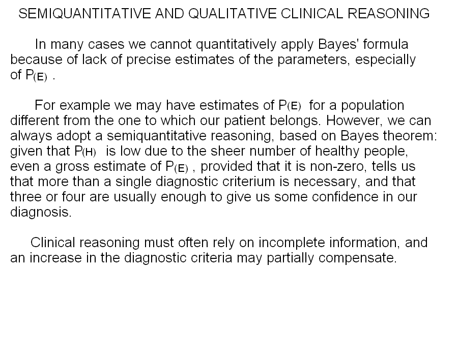
In many cases we cannot quantitatively apply Bayes' formula because of lack of precise estimates of the parameters, especially of P(E). For example we may have estimates of P(E) for a population different from the one to which our patient belongs. However, we can always adopt a semiquantitative reasoning, based on Bayes theorem: given that P(H) is low due to the sheer number of healthy people, even a gross estimate of P(E), provided that it is non-zero, tells us that more than a single diagnostic criterium is necessary, and that three or four are usually enough to give us some confidence in our diagnosis. Clinical reasoning must often rely on incomplete information, and an increase in the diagnostic criteria may partially compensate.
Differential diagnosis
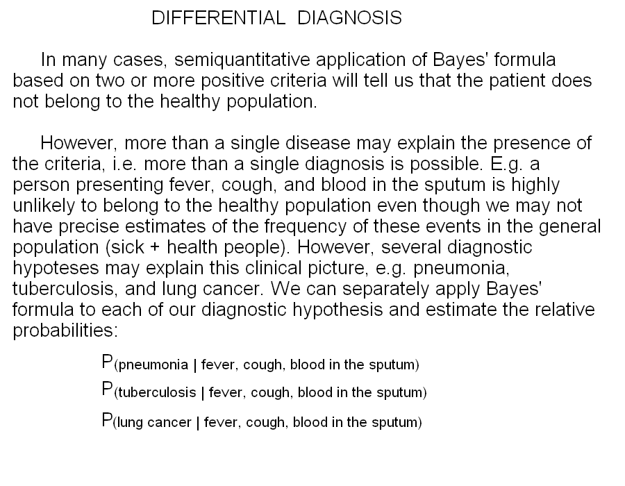
In many cases, semiquantitative application of Bayes' formula based on two or more positive criteria will tell us that the patient does not belong to the healthy population. However, more than a single disease may explain the presence of the criteria, i.e. more than a single diagnosis is possible. E.g. a person presenting fever, cough, and blood in the sputum is highly unlikely to belong to the healthy population even though we may not have precise estimates of the frequency of these events in the general population (sick + health people). However, several diagnostic hypoteses may explain this clinical picture, e.g. pneumonia, tuberculosis, and lung cancer. We can separately apply Bayes' formula to each of our diagnostic hypothesis and estimate the relative probabilities: P(pneumonia|fever, cough, and blood in the sputum), P(tuberculosis|fever, cough, and blood in the sputum) and P(lung cancer|fever, cough, and blood in the sputum).
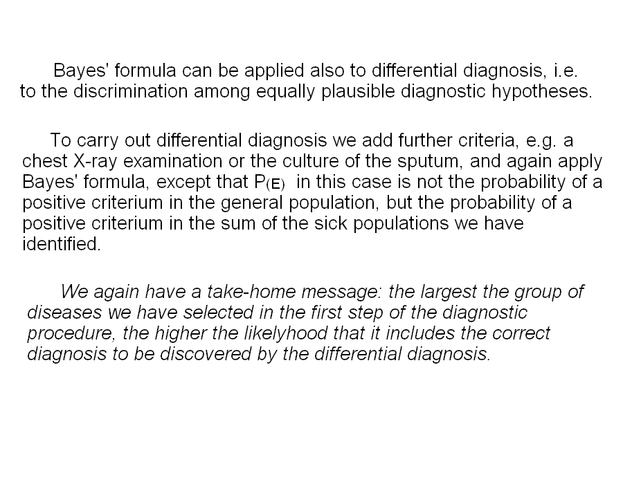
In some cases one hypothesis will be overwhelmingly more likely than the others; in other cases further investigation will be required. Bayes' formula can be applied also to differential diagnosis, i.e. to the discrimination among equally plausible diagnostic hypotheses. To carry out differential diagnosis we add further criteria, e.g. a chest X-ray examination or the culture of the sputum, and again apply Bayes' formula, except that P(E) in this case is not the probability of a positive criterium in the general population, but the probability of a positive criterium in the sum of the sick populations we have identified.
We again have a take-home message: the largest the group of diseases we have selected in the first step of the diagnostic procedure, the higher the likelyhood that it includes the correct diagnosis to be discovered by the differential diagnosis.
THRESHOLDS
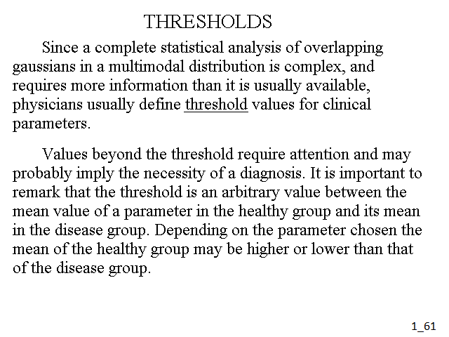
Since a complete statistical analysis of overlapping gaussians in a multimodal distribution is complex, and requires more information than it is usually available, physicians usually define threshold values for clinical parameters. Values beyond the threshold require attention and may probably imply the necessity of a diagnosis. It is important to remark that the threshold is an arbitrary value between the mean value of a parameter in the healthy group and its mean in the disease group. Depending on the parameter chosen the mean of the healthy group may be higher or lower than that of the disease group. Thus in some cases (e.g. the IQ) the presence of illness is more likely if the parameter value is below the threshold; in other cases (e.g. bilirubin concentration in the blood) the presence of illness is more likely if the parameter value is above the threshold.
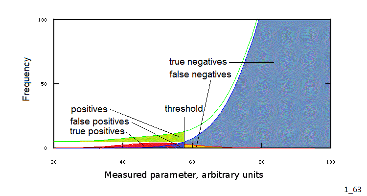
As evident from Fig.3 any threshold value will include members from the healthy group and/or exclude members of the disease group. E.g. suppose that we take IQ=55 as a sensible threshold, implying that any individual with IQ<55 requires further study: this threshold will exclude 20% of the members of the disease group, having IQ>55, who will not be further studied and thus wil not be diagnosed, and 0.05% of the members of the healthy group, for whom a diagnosis will be uselessly searched for.
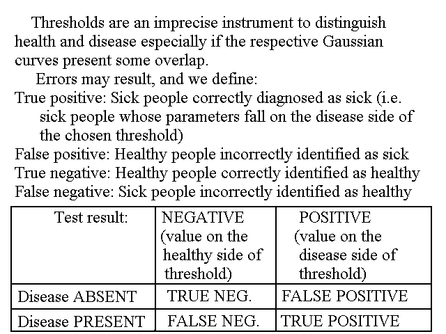
In the clinical jargon we call positive (i.e. potentially ill) all values falling on the "unexpected" side of the chosen threshold (e.g. IQ<55); positive values may or may not be due to illness and negative values may or may not be associated to health: we call true positives the values on the unexpected side of the threshold that when further indagated lead to a diagnosis and false positives those which do not lead to a diagnosis. In the same way we call negative all values on the "expected" side of the threshold; true negatives if no illness is present, false negatives in the opposite case. In summary:
True positive: Sick people correctly diagnosed as sick
False positive: Healthy people incorrectly identified as sick
True negative: Healthy people correctly identified as healthy
False negative: Sick people incorrectly identified as healthy
| Test result: NEGATIVE (value on the expected side of the threshold) |
Test result: POSITIVE (value on the unexpected side of the threshold) | |
| DISEASE ABSENT | TRUE NEGATIVE | FALSE POSITIVE |
| DISEASE PRESENT | FALSE NEGATIVE | TRUE NEGATIVE |

Fig.4: Positive and negative test results
The existence of false positives and false negatives is obviously unpleasant: medicine would be simpler if we could eliminate these and unequivocally associate positive to illness and negative to health. This occurs in the cases described above of certainty diagnoses, and depends on a negligible or absent overlapping of the gaussian distribution of clinical parameter values' in the healthy and disease groups. In all other condition, however false positives and false negatives occur. By accurately deciding the threshold value we can reduce and even abolish either false result, but at the expense of an increase of the frequency of the other false result. E.g. in the case of the IQ we can minimize the frequency of false negatives by increasing the threshold to IQ=80, but such a high threshold will cause a high frequency of false positives (refer to Figs.3 and 4).
SENSITIVITY AND SPECIFICITY OF TESTS
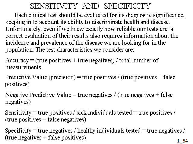
Each clinical test should be evaluated for its diagnostic significance, keeping in to account its ability to discriminate health and disease. Unfortunately, even if we knew exactly how reliable our tests are, a correct evaluation of their results also requires information about the incidence and prevalence of the disease we are looking for in the population. The test characteristics we consider are:
Accuracy = (true positives + true negatives) / total number of measurements.
Predictive Value (precision) = true positives / (true positives + false positives)
Negative Predictive Value = true negatives / (true negatives + false negatives)
Sensitivity = true positives / sick individuals tested = true positives / (true positives + false negatives)
Specificity = true negatives / healthy individuals tested = true negatives / (true negatives + false positives)
These characteristics are not independent from each other: e.g. sensitivity and specificity depend on the same threshold, thus one cannot increase the one without decreasing the other. More refined correlations may be written down if one knows the prevalence of the disease in the population:
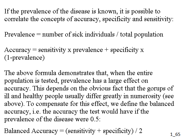
Prevalence = number of sick individuals / total population
E.g. accuracy estimates how often the test yields a true result, be it positive or negative, and, if the entire population (or a large random sample) has been tested, bears the following relation to specificity and sensitivity:
Accuracy = sensitivity x prevalence + specificity x (1-prevalence)
The above formula demonstrates that, when the entire population is tested, prevalence has a large effect on accuracy. This depends on the obvious fact that the gorups of ill and healthy people usually differ greatly in numerosity (see above). To compensate for this effect, we define the balanced accuracy, i.e. the accuracy the test would have if the prevalence of the disease were 0.5:
Balanced Accuracy = (sensitivity + specificity) / 2
| Characteristics of test | Suggested use | test positive | test negative |
| high accuracy (few false + and false -) | All | Probably sick | Probably healthy |
| high sensitivity low specificity (few false -) | Secondary prevention (large scale screening) | Possibly sick (investigate further) | Probably healthy |
| high specificity low sensitivity (few false +) | Diagnostic tool | Probably sick | Possibly healthy (investigate further if necessary) |
UNDESIRABLE NORMAL CONDITIONS; MORAL AND ECONOMICAL CONSIDERATIONS
All the above considerations deal with the hypothesis that sick and healthy people belong to two different groups of the population, and that each patient can be assigned to his or her proper group by means of the opportune clinical tests. There may be, however, conditions that are undesirable and entail an unfavorable prognosis even thoough they fully belong to the "normal" range of parameters. Since these conditions can often be treated it is important to recognize them. An example is hypercholesterolemia. There are several diagnosticable genetic diseases that cause such condition. However, also in the absence of any of these, there are individuals whose blood cholesterol concentration is high . These individuals represent the tail of a Gaussian distribution and properly speaking do not require a diagnosis: they are healthy individuals whose blood cholesterol concentration is 2 or 3 SD above the mean value. In spite of belonging to the normal population, these individual risk all the unwanted consequences of hypercholesterolemia, as ill people do: i.e. the complications of hypercholesterolemia (e.g. atherosclerosis) do not depend on the genetic disease that may or may not be present, but on the actual concentration of cholesterol in the blood. Thus people whose blood cholesterol exceeds some consensus value (240 to 280 mg/dL) should be treated even in the absence of a genetic diagnosis of hereditary hypercholesterolemia. It is important that the physician is aware of the conceptual difference of diagnosing and treating the members of the disease group or the tails of the healthy group Gaussian.
The use made above of the concepts of health and disease implies some ethical considerations: indeed if an individual belongs to the healthy group and yet his or her clinical parameters present severe deviations from the average values, one may consider whether he needs therapy nevertheless. There is no general rule on this point, but the widespread consensus holds that if an effective symptomatic therapy exists this should be extended to all individuals who may benefit from it, whereas causal therapies should be prescribed, and will only function, according to the diagnosis. E.g. all people with an IQ<50 (or 70) may greatly benefit from receiving specific attention and care by specifically trained staff, at school and elsewhere, irrespective of the diagnosis; on the other hand a specific therapy will benefit only people suffering of a given disease (e.g. a diet low in phenylalanine and tyrosine is a specific cure of phenylketonuria and the low IQ due to this disease, but will not cure other clinical conditions).
Ethics is also to be considered in the case of thresholds: if we are dealing with a lethal but curable disease (e.g. appendicitis; typhoid; most early cases of cancer; etc.) it is sensible to minimize false negatives by setting a threshold closer to the mean of true negatives. This is because the consequences of neglecting a diagnosis may be fatal, whereas the increase of false positives will only cause to these patients the inconvenience of further analyses which will confirm that the disease is not present. However, the physician must use great care to avoid an unnecessary intervention: e.g. operating a false positive for appendicitis.
Home of this course
Slides of this lecture:
 |
 |
 |
 |
 |
 |
 |
 |
 |
 |
 |
 |
 |
 |
 |
 |
 |
 |
 |
 |
 |
 |
 |
 |
 |
 |
 |
 |
 |
 |
 |
 |
 |
 |
 |
 |
 |
 |
 |
 |
 |
 |
 |
 |
 |
 |
 |